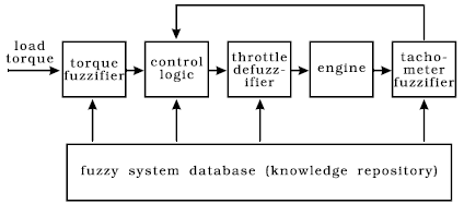
Fig. 5.9: Adaptive fuzzy-logic vehicle engine control system block diagram
Fuzzy logic control systems are particularly interesting as mixed-signal systems. Engineers often use general-purpose mathematical packages to develop fuzzy logic control systems. However, those systems eventually end up in hardware, when electronic circuit simulators should be used. Due to AleC++ modeling power, Alecsis is capable of supporting the entire design process, from the conceptual to the final stage. The example of such a system may be an adaptive fuzzy-logic vehicle engine controller, shown in Fig. 5.9.
Fig. 5.9: Adaptive fuzzy-logic vehicle engine control system block diagram
The system controls a vehicle engine in order to respond to changes in the road grade [Cox93]. The engine speed is monitored using a tachometer. In order to solve the control problem using the fuzzy-logic approach, the tachometer readings and the road grade are first fuzzyfied. This information is used to produce a fuzzyfied engine throttle movement value in the control logic block. The exact (crisp) control value is obtained in the defuzzyfication module, and then applied to the engine. As expected, the entire system is parameterized by creating a new model class, containing data about fuzzy regions, domain knowledge in the form of a fuzzy associative matrix, rule weights and so on. Connections between the modules are modeled using variables of type flow for crisp values, and structures for fuzzy values. The entire system is self-adaptive, i.e. capable of responding to long-range changes in the environment. The behavior of all of the modules is implemented as model class methods, including the self-adaptation mechanism. The vehicle engine was modeled using an ordinary differential equation by means of AleC++ eqn statement.
The first step in modeling for Alecsis is to create a new class that describes resources needed in the simulation:
class fuzzy {
int ntach; // number of tachometer fuzzy values
int nlt; // number of load torque fuzzy signals
int ntas; // number of throttle mov. fuzzy values
FUZZY_VALUE tach[TACHSIZE]; // tachometer fuzzy logic system
FUZZY_VALUE torq[LTSIZE]; // load torque fuzzy logic system
FUZZY_VALUE tas[TMSIZE]; // throttle action fuzzy log. sys.
double tcmin, tcmax; // tachometer range
double trqmin, trqmax; // load torque range
double tamin, tamax; // throttle action range
int fam[LTSIZE][TACHSIZE];// fuzzy assoc. memory (knowledge)
int center_of_response[2];// steady-state location
double weights[LTSIZE][TACHSIZE]; // FAM weights matrix
void fuzzy(int); // class constructor
void ~fuzzy(int); // class destructor
double engine_response; // engine reaction
public:
double memf(FUZZY_VALUE*,double,double); // membership func.
void evaluate_output(double*,double*,double*,int);// mapping
double integrate(double*); // evaluation of centroid
void update_weights(); // auto-adaptation of weights
};
After the definition of the model class, an unlimited number of model cards of that class may be constructed. An example may look like this:
model fuzzy::speed_cont {
ntach=5; nlt=4; ntas=5; tcmin=0.1; tcmax=8.0;
trqmin=0; trqmax=40; tamin=-60; tamax=60;
// tachometer fuzzy value system coordinates (feedback)
tach = { { "very_slow", { 0.1, 0.1, 0.4, 0.8 } },
{ "slow", { 0.5, 1.65, 1.65, 2.8 } },
{ "optimal", { 2.0, 3.25, 3.25, 4.5 } },
{ "fast", { 3.2, 4.7, 4.7, 6.2 } },
{ "very_fast", { 5.5, 7.0, 8.0, 8.0 } } };// load torque fuzzy value system coordinates (feed forward)
torq = { { "zero", { 0, 0, 2.5, 10 } },
{ "small_positive", { 5, 12.5, 12.5, 20 } },
{ "moderate_positive", { 15, 22.5, 22.5, 30 } },
{ "large_positive", { 25, 32.5, 40, 40 } } };// throttle action fuzzy value system coordinates (output)
tas = { { "LN", { -60, -60, -45, -30 } },
{ "SN", { -40, -20, -20, -2 } },
{ "ZR", { -10, 0, 0, 10 } },
{ "SP", { 2, 20, 20, 40 } },
{ "LP", { 30, 45, 60, 60 } } };// fuzzy associative memory (knowledge repository)
fam = { { LP, SP, ZR, SN, LN },
{ LP, SP, ZR, ZR, SN },
{ LP, SP, SP, SP, ZR },
{ LP, LP, LP, SP, SP } };// initial equilibrium center on the control surface
center_of_response = {Optimal, Zero };
// initial rule contribution weights - all rules are equal
weights = { { 1, 1, 1, 1, 1 },
{ 1, 1, 1, 1, 1 },
{ 1, 1, 1, 1, 1 },
{ 1, 1, 1, 1, 1 } };
}
Fig. 5.10: Vehicle engine control system response to rapid change in the road grade
Fig. 5.10 shows the system response to a rapid change in the road grade. Two distinct regions exist in the response curve: one, that represents the primary response, and another, where the system slowly adjusts the rule weights to move the center of the response to a different location. This effect is shown in the weight surfaces in the Fig. 5.11. The center-of-response displacement is clearly visible on the surface contour lines.
Fig. 5.11: Weight surfaces before (a) and after (b) the road grade change. The center of response has visibly moved towards the new equilibrium point.